The subtle part of the subject lies in understanding what computation to ask the computer to do for you—it is far less important to know how to perform computations that a computer can do better than you anyway.
Here is the row reduction algorithm, summarized in pictures.
Definition
Reflections
Reflection in the y-axis
Reflection in the x-axisReflection in the origin
Rotation about the origin
Scaling Skewing (shearing) in the x- and y-directions
Translation in the x- and y-directions
It will be very important to know where are the pivots of a matrix after row reducing; this is the reason for the following piece of terminology.
A pivot position of a matrix is an entry that is a pivot of a row echelon form of that matrix.
A pivot column of a matrix is a column that contains a pivot position.
My own opinion, we are just flat landers in 3D.
It is very hard to understand Linear Transformation with Vectors space with more than 3 Dimension, but it is very easy to understand them with 2D and 3D. You can watch the below video if you like to know why.
Linear transformations are divided into the following types.
a. Rigid transformations (distance preserving)
Rigid transformations leave the shape, lengths and area of the original object unchanged. Rigid transformations are:
Translation
Rotation
b. Similarity transformations (angle preserving)
Similarity transformations preserve the angles of the original object, but not necessarily the size. Similarity transformations are:
Translation
Rotation
Uniform scale (the same amount of scale in the x- and y-directions)
c. Affine transformations (parallel preserving)
Affine transformations preserve any parallel lines, but may change the shape and size. Affine transformations are:
Translation
Rotation
Scale
Skew (shear)
Notice Rigid transformations are a subset of Similarity transformations, which are in turn a subset of Affine transformations.
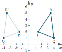
Make x = -x
Transforming Matrix may look line [-1, 0;
0, 0]
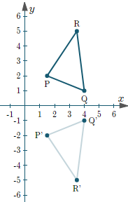
Make y = -y.
Transforming Matrix may look line [1, 0;
0, -1]
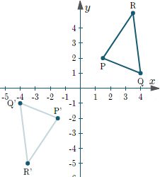
Make x = -x and y = -y
Transforming Matrix may look line [-1, 0;
0, -1]
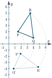
Make use of trigonometry to rotate the triangle with cosines and sines.
Transforming Matrix may look line [cos(theta), sin(theta);
- sin(theta), cos(theta)]
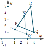
make x = a.x and y = b.y
Transforming Matrix may look line [a, 0;
0, b]
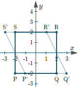
Transforming Matrix may look line [1, -tan(theta);
0, 1] or
[1, 0;
-tan(theta), 1]
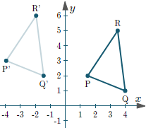
We cannot achieve translation using 2×2 matrices. we need to take 3x3 to achieve this.
Transforming Matrix may look line [1, 0 a;
0, 1 0;
0, 0, 1]
or
Transforming Matrix may look line [1, 0 0;
0, 1 b;
0, 0, 1]
In general, a transformation F is a linear transformation if for all vectors v1 and v2 in some vector space V, and some scalar c,
F(v1 + v2) = F(v1) + F(v2); and
F(cv1) = cF(v1)
transforming the map with 3 vectors pointing to 3 places in Australia and scaling and
skewing Australian map only with the change in Eigen Value and in the matrix,
they are changing the value in the non primary diagonal of matrix.
With SkewXY he is scaling and skewing the map with 2 Vectors instead of 1
Vector denoting one place in Australia.
And then allows us to skew the map first with X and then with Y sequentially,
one after the other independently.
Here is a summary of the rules that governs reflection, rotation, translation and dilation / scaling

Scaling is also called as Dilation transformation, it looks as one of the most important
transformation as our eyes also dilates few this with it focus.
Once you have understood linear transformation and eigen vectors then take off from here to understand more dimension considering only vectors in spaces.
References:


No comments:
Post a Comment